Language Modeling with Hyperspherical Flows
Recent continuous flow language models (FLMs) operate on one-hot vectors and perform similarly to AR models in Generative Perplexity. However, FLMs are costly to train. Additionally, while Gaussian noise on images smoothly destroys information from high to low frequencies, its effect on one-hot vectors is not as clear. Instead of Gaussian noise, we propose a different noise process, better suited to token representations. We inject noise by rotating unit-norm embeddings on $\mathbb{S}^{d-1}$. On GSM8k, where prior FLMs fail, we approach the quality of discrete diffusion models. At the same time, a large gap with AR models remains.
Justin Deschenaux · Caglar Gulcehre · EPFL
Created May 13, 2026
Autoregressive (AR) models dominate language modeling. AR models implemented with causal transformers are efficient to train and scale to billions of parameters:
$$p(x_1, \ldots, x_N) = \prod_{i=1}^{N} p(x_i \mid x_{\lt i}).$$
During sampling, AR models must generate tokens one-by-one, which is slow. Causal attention is also poorly suited for reasoning tasks where bidirectional context matters.
Discrete diffusion language models (such as MDLM and Duo) enable parallel generation with bidirectional context, and approach AR in Generative Perplexity (the perplexity of generated samples, measured by a large AR model). At every denoising step, however, tokens are drawn from a factorized distribution for tractability. The factorization makes discrete diffusion less expressive than AR when sampling in parallel.
Continuous flows trained with Flow Matching learn a velocity field $u_t^\theta$ that defines an ODE transporting noisy samples $z_0 \sim p_0$ to the data distribution $p_1$:
$$\frac{d}{dt}\phi_t(z_0) = u_t^\theta\bigl(\phi_t(z_0)\bigr), \qquad \phi_0(z_0) = z_0.$$
During inference, all positions are updated jointly, and integrating the ODE produces a sample. Recent flow language models (FLMs) (Lee et al., Roos et al., Potaptchik et al.) learn a standard Gaussian flow on one-hot token representations. We propose the Hyperspherical Flow Language Model ($\mathbb{S}$-FLM), a Riemannian flow on the unit sphere that learns embeddings end-to-end, does not rely on Gaussian noise, and does not materialize huge one-hot vectors. One important question motivating $\mathbb{S}$-FLMs is:
Is Gaussian noise the right choice for flow language modeling?
1. Motivation
Recent flow language models add Gaussian noise to one-hot vectors, producing dense tensors that are costly to store and process. Instead, we train the denoiser to recover the clean token from a rotated embedding.
Recent flow language models (Lee et al., Roos et al., Potaptchik et al.) represent tokens as one-hot vectors, add Gaussian noise, and train with cross-entropy. They match the Generative Perplexity of autoregressive and discrete diffusion models, but have a few shortcomings.
(1) Materializing large one-hot vectors is costly. Modern LLMs commonly use vocabularies containing 100k–200k tokens, so storing one-hot vectors is costly at scale. After adding Gaussian noise, the denoiser multiplies those vectors by the token embedding matrix instead of looking up a single row, which makes FLMs slower to train than discrete diffusion and AR models.
(2) Gaussian noise on one-hot vectors is hard to interpret. On images, Gaussian diffusion smoothly degrades higher-frequency components first. For one-hot vectors, the interpretation of adding Gaussian noise is not as clear.
The hypersphere, by contrast, has several desirable properties. First, the cosine distance is more suited than the Euclidean distance for comparing word embeddings (word2vec, GloVe). Secondly, replacing the Gaussian prior of VAEs with a hyperspherical one can improve performance (Davidson et al.). Lastly, nGPT constrains the activations and weights of an AR model to be on $\mathbb{S}^{d-1}$, which improves the training stability.
(3) FLMs on one-hot vectors underperform on reasoning tasks. While previous FLMs perform well on sudoku, when the vocabulary size grows, eg ~50k, their accuracy on GSM8K is close to zero, while AR achieves 50-60%.
We therefore propose the Hyperspherical Flow Language Model ($\mathbb{S}$-FLM), a flow over embeddings that does not need to materialize one-hot vectors. Since the cosine distance is determined by the arc length on $\mathbb{S}^{d-1}$, we implement $\mathbb{S}$-FLM as a Riemannian flow on $\mathbb{S}^{d-1}$. On GSM8k, $\mathbb{S}$-FLM reaches up to 18% accuracy, while FLMs on one-hot vectors are below 0.5%.
2. Method
Tokens are learnable unit-norm vectors on . Training: we rotate clean embeddings toward random points on the sphere and train a denoiser with cross-entropy. Sampling: at each step, the velocity is a weighted average of the tangent directions toward each clean embedding. On the last step, we decode with . Careful design of the noise schedule is necessary.
2.1 Training: SLERP on the sphere
Each token $v \in \mathcal{V}$ is associated with a unit-norm embedding $\hat{\mathbf{e}}_v = \mathbf{e}_v / \|\mathbf{e}_v\| \in \mathbb{S}^{d-1}$, where $\mathbf{e}_v$ is the $v$-th row of an embedding table $\mathbf{E} \in \mathbb{R}^{|\mathcal{V}| \times d}$. At every position $\ell$ in the sequence, we take $\mathbf{z}_1^\ell = \hat{\mathbf{e}}_{x^\ell}$, draw $\mathbf{z}_0^\ell \sim \mathcal{U}(\mathbb{S}^{d-1})$, and form the noisy latent with spherical linear interpolation (SLERP):
$$ \mathbf{z}_t^\ell = \mathrm{SLERP}(\mathbf{z}_0^\ell, \mathbf{z}_1^\ell, \alpha_t) = \frac{\sin((1-\alpha_t)\omega)}{\sin\omega}\,\mathbf{z}_0^\ell + \frac{\sin(\alpha_t\,\omega)}{\sin\omega}\,\mathbf{z}_1^\ell, $$
where $\omega = \arccos(\mathbf{z}_0^{\ell\top} \mathbf{z}_1^\ell)$ is the angle between $\mathbf{z}_0^\ell$ and $\mathbf{z}_1^\ell$.
Unlike standard flow matching on fixed data (such as pixels), we train $\mathbf{E}$, the data representation, jointly with the flow by backpropagating through the SLERP. Concretely, we train a denoiser $p^\theta_{1|t}$ with cross-entropy:
$$ \mathcal{L}_{\text{CE}}(\theta) = \mathbb{E}_{\mathbf{x} \sim p_1,\, t \sim \mathcal{U}[0,1],\, \mathbf{z}_0 \sim p_0} \left[ -\sum_{\ell=1}^L \log p^\theta_{1|t}(x^\ell \mid \mathbf{z}_t) \right]. $$
2.2 Sampling: marginalize the conditional velocities
Flow Matching parameterizes the velocity field $u_t$ as an expectation over conditional velocities $u_{t \mid 1}$:
$$ u_t(\mathbf{z}_t^\ell) = \int u_{t \mid 1}(\mathbf{z}_t^\ell \mid \mathbf{z}_1^\ell)\, p_{1 \mid t}(\mathbf{z}_1^\ell \mid \mathbf{z}_t^\ell)\, d\mathbf{z}_1^\ell. $$
For us, $u_{t \mid 1}$ is the time-derivative of SLERP, a tangent vector at $\mathbf{z}_t^\ell$ pointing toward the clean embedding. Because the data is discrete, the expectation reduces to a sum over elements of the vocabulary $\mathcal{V}$:
$$ u_t(\mathbf{z}_t^\ell) = \sum_{v \in \mathcal{V}} u_{t \mid 1}(\mathbf{z}_t^\ell \mid \hat{\mathbf{e}}_v)\, p_{1 \mid t}(v \mid \mathbf{z}_t^\ell). $$
Substituting the closed-form expression for $u_{t \mid 1}$ (derivative of SLERP) and using the trained posterior $p^\theta_{1|t}$ gives the exact velocity:
$$ u^\theta_t(\mathbf{z}_t^\ell) = \frac{\dot{\alpha}_t}{1 - \alpha_t} \sum_{v \in \mathcal{V}} p^\theta_{1|t}(v \mid \mathbf{z}_t^\ell)\, \log_{\mathbf{z}_t^\ell}(\hat{\mathbf{e}}_v). $$
Here, $\log_{\mathbf{z}_t^\ell}(\hat{\mathbf{e}}_v)$ is the logarithmic map, a standard construction from Riemannian geometry on manifolds. For our purposes, it is the tangent vector at $\mathbf{z}_t^\ell$ pointing toward $\hat{\mathbf{e}}_v$ along the geodesic.
As in Euclidean Flow Matching, we generate samples by integrating the ODE
$$ \frac{d\mathbf{z}_t^\ell}{dt} = u^\theta_t(\mathbf{z}_t^\ell), \qquad t \in [0, 1], $$
starting from a random point $\mathbf{z}_0^\ell \sim \mathcal{U}(\mathbb{S}^{d-1})$ on the sphere at $t = 0$ and ending at a clean embedding $\mathbf{z}_1^\ell$ at $t = 1$. On the sphere, each integration step is a small rotation along the velocity field.
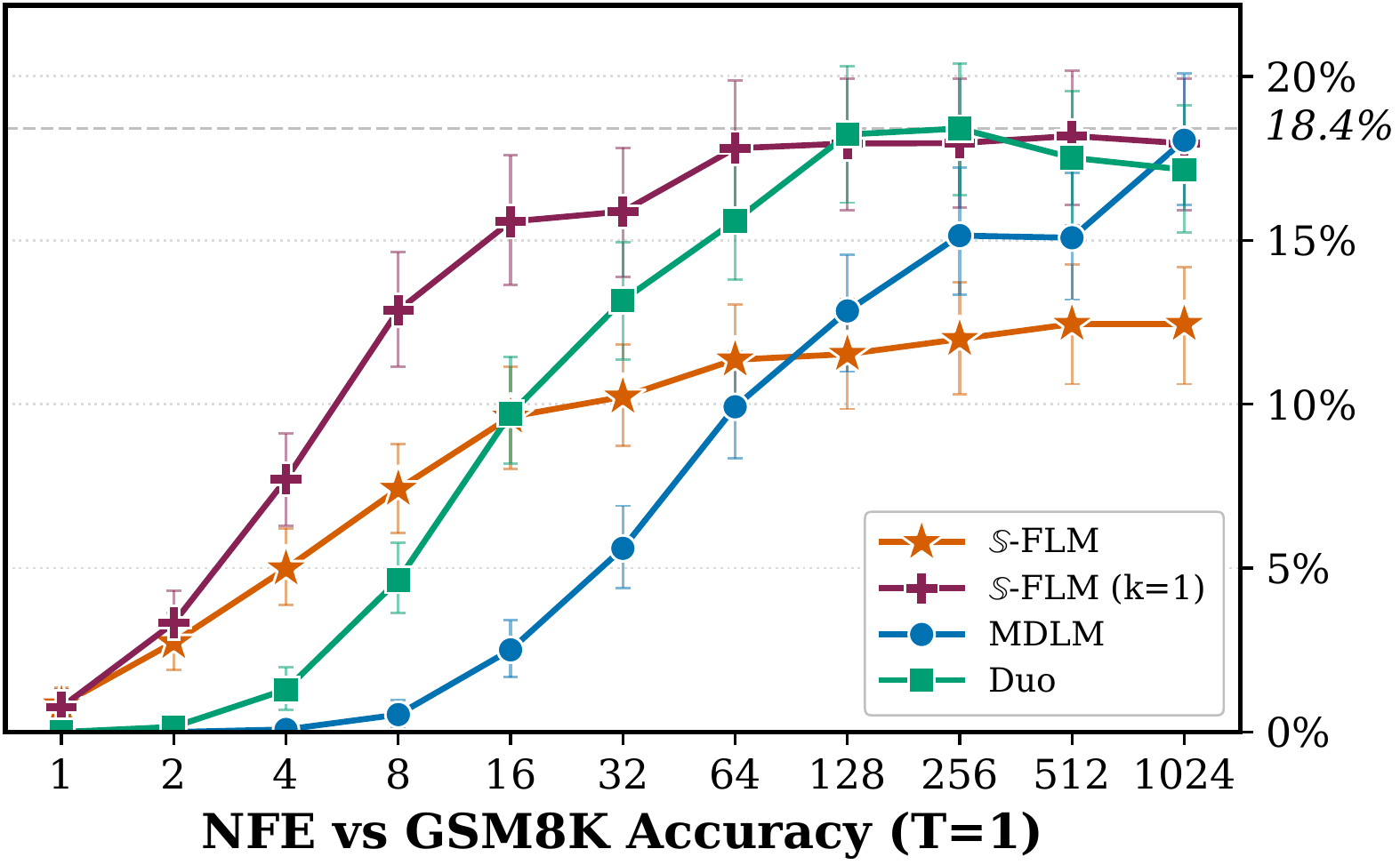
We experiment with two alternatives: replace the sum with a single Monte Carlo sample of $p^\theta_{1|t}$ (stochastic decoding), or restrict it to the top-$k$ entries (top-$k$ velocity decoding). Top-$1$ is the analogue of greedy autoregressive decoding, and on GSM8k it closes the gap to MDLM and Duo at $T = 1$.
Three candidate clean embeddings (), a noisy sample , and the three tangent vectors at pointing toward each clean vector. The marginal velocity is a weighted sum of the tangent vectors.
2.3 Truncating the noise schedule
Recall that $\alpha_t = 0$ is pure noise and $\alpha_t = 1$ is the clean embedding. When $\alpha_t$ is close to 1, the sample $\mathbf{z}_t^\ell$ is already close to the clean embedding and the true posterior $p_{1|t}$ is close to one-hot: with small rotations and well-separated embeddings, the nearest clean embedding is obvious. Training at these $\alpha_t$ values is a waste of compute, since the denoising task is easy. We therefore truncate the schedule and only train at $\alpha_t \in [0, \alpha^\star(\delta)]$, the noisier values where the denoiser actually has to work. The question is: how to choose $\alpha^\star(\delta)$?
Under a simplified model of the sampling dynamics (geodesic interpolation from $\mathbf{z}_0^\ell$ to a clean embedding, with embeddings drawn i.i.d.\ from $\mathcal{U}(\mathbb{S}^{d-1})$), we derive a closed-form expression for $\alpha^\star(\delta)$, the smallest $\alpha$ at which the target is the nearest neighbor of $\mathbf{z}_\alpha$ with probability at least $1 - \delta$:
$$ \alpha^\star(\delta) \approx \frac{2}{\pi}\, \arcsin\!\left(\sqrt{\frac{2 \log(2(|\mathcal{V}|-1)/\delta)}{d}}\right). $$
Truncating to $[0, \alpha^\star(\delta)]$ improves the accuracy on GSM8k from 1.2% to 7.7% and on Sudoku (hard) from 14.0% to 43.2%.
Voronoi cells of the clean embeddings are shown in color. The derivation of above is inspired by finding the smallest at which the sampling trajectory enters the target's Voronoi cell, under a simplified model with i.i.d. uniform embeddings.
2.4 Adaptive noise schedule
In addition to truncating the noise schedule, we also make its "shape" adaptive. Inspired by InfoNoise, every 50 optimizer steps we fit the recent time / loss value pairs $(t, \mathcal{L})$ with ridge regression to get $\hat{\mathcal{L}}(t)$, and set $\alpha_t$ to the inverse CDF of $|d\hat{\mathcal{L}}/dt|$. By inverse-transform sampling, a uniform $t \in [0, 1]$ maps to an $\alpha_t$ drawn from the density $|d\hat{\mathcal{L}}/dt|$. This enables sampling more frequently at noise levels where the loss is decreasing the most. Since we fit the loss relatively frequently, we smoothen the schedule by using an exponential moving average.
Drag the sliders to move and sharpen the loss-derivative peak. The schedule flattens where is largest, so uniform samples cluster around the peak.
2.5 A hyperspherical backbone
The latents $\mathbf{z}_t^\ell$ live on $\mathbb{S}^{d-1}$ and the sampling step rotates them. Inspired by nGPT, we adapt the transformer block so that each MLP and self-attention layer also rotates its input. We call the resulting backbone 𝕊-arch. For time conditioning, we adapt the rotation angle based on the noise level, analogous to adaptive layer norms in DiT. The 𝕊-arch has slightly fewer parameters than the standard DiT used in discrete-diffusion papers because the time conditioning is lighter.
3. Results
-FLM performs similarly to previous FLMs on Sudoku Hard. On GSM8k, where prior FLMs are below 0.5%, -FLM reaches up to 18%. Still, a large gap to AR (50-60%) remains.
Accuracy on Sudoku Hard and GSM8k
For GSM8k, we differentiate between the exact and top-1 velocities.
Sudoku Hard
exact-match %GSM8k
accuracy %3.1 Sudoku
On hard Sudoku puzzles (30 visible digits), we use a large number of sampling steps to measure the maximum achievable performance. The vanilla 𝕊-FLM reaches 14.0%. Truncation increases the accuracy to 43.2%, and the adaptive schedule reaches 45.0%, comparable to the prior best continuous model. Duo is best at 58.4%.
3.2 GSM8k
Prior continuous FLMs (CANDI, one-hot FLM) reach less than 0.5% on GSM8k. With the vanilla linear schedule , 𝕊-FLM already beats them at 1.2%. Truncation increases the accuracy to 7.7%, the adaptive schedule to 11.1%, and the 𝕊-arch backbone to 12.4%. Top-1 velocity decoding reaches 18.0% at , matching MDLM and Duo. At , the exact-velocity variant of 𝕊-FLM beats both.
3.3 OpenWebText
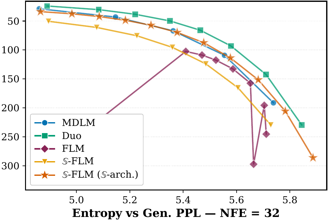
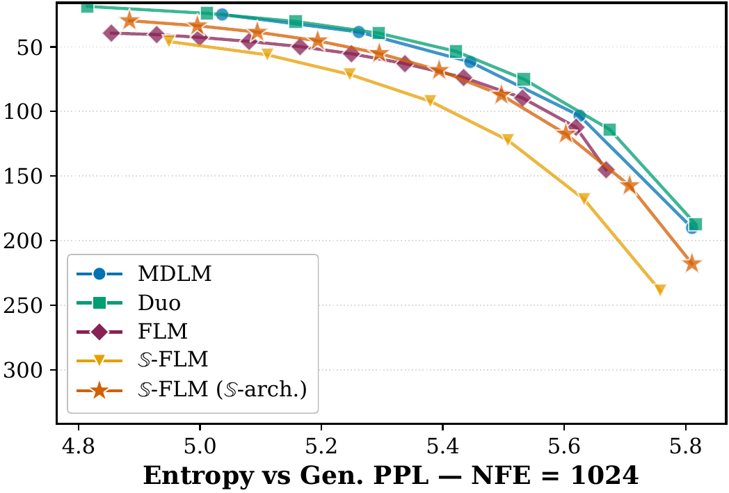
We plot the Gen.PPL / entropy frontier by sweeping the sampling temperature. At , 𝕊-FLM matches prior FLMs. At , the Pareto frontier of prior FLMs becomes unstable while 𝕊-FLM stays comparable to MDLM.
4. Conclusion
-FLM matches the prior best continuous FLMs on Sudoku and exceeds them on GSM8k, while training faster because it never materializes -dimensional one-hot vectors. A clear gap to autoregressive models remains on GSM8k.
We introduced $\mathbb{S}$-FLM, a Riemannian flow on the unit sphere that learns its velocity field and token embeddings jointly. All recent continuous-diffusion attempts at language modeling use Gaussian noise, which we think is not necessarily best suited to token representations. The other contributions are the $\mathbb{S}$-arch backbone with normalized activations and the truncated, adaptive noise-schedule analysis.
On Sudoku, $\mathbb{S}$-FLM performs similarly to prior FLMs. On GSM8k, where the accuracy of all previous FLMs is below $0.5\%$, $\mathbb{S}$-FLM with top-$1$ decoding closes the gap to MDLM and Duo at $T = 1$, though a gap remains at low-temperature ($T = 0.1$) sampling. On OpenWebText, $\mathbb{S}$-FLM follows the Gen.PPL / entropy frontier of prior FLMs at high NFE and stays stable at low NFE where prior continuous models do not.
Because $\mathbb{S}$-FLM never materializes a $|\mathcal{V}|$-dimensional one-hot vector, it trains faster than prior FLMs and may be easier to scale, though we leave that to future work. The truncation bound we derive provides a principled heuristic that works well in practice. A clear gap between continuous diffusion and autoregressive models remains on GSM8k.
5. BibTeX
@misc{deschenaux2026languagemodelinghypersphericalflows,
  title         = {Language Modeling with Hyperspherical Flows},
  author        = {Justin Deschenaux and Caglar Gulcehre},
  year          = {2026},
  eprint        = {2605.11125},
  archivePrefix = {arXiv},
  primaryClass  = {cs.LG},
  url           = {https://arxiv.org/abs/2605.11125}
}